Vision LLM · Appearance QC / Feasibility Plan
Home Appliances: Ring Outer-Edge Chip Inspection — Feasibility Study
A Φ34.46 mm alloy ring, both faces, 360° of outer rim— dome diffuse light turns a chip into a silhouette problem, and unwrapping the rim into a radius curve turns the verdict from “does it look like a defect” into “how many millimetres are missing”.
Key takeaways
- A chip is geometry, not texture. Dome diffuse lighting blows the alloy face to uniform white and keeps the background dark, so oil film and turning marks stop mattering. What is left is one silhouette of the outer circle—and the criterion moves from grey level to geometry.
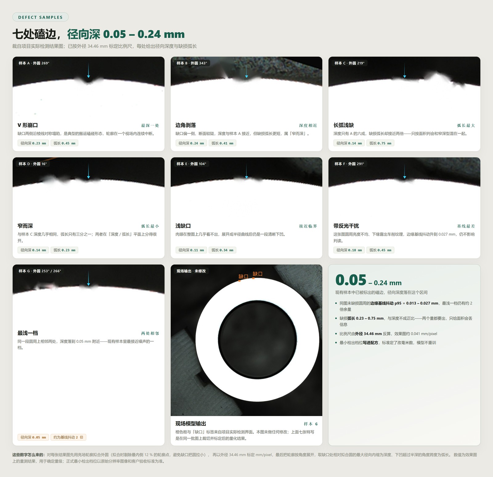
- Measure the existing result images first. Scaling by the known 34.46 mm outside diameter, the seven marked chips run 0.05 – 0.24 mm deep radially and 0.23 – 0.75 mm along the arc, while the intact rim in the same frames sits within a 0.013 – 0.027 mm P95 baseline jitter.
- The whole rim fits in one frame. Five megapixels over a 42 mm field is 0.020 mm/pixel, spreading the 108 mm circumference across about 5300 pixels. No stitching, no rotary stage—and therefore no seams and no re-positioning error.
- Three-centre alignment is about lighting, not centring. Lateral offset and height variation are absorbed by fitting the circle per frame; the one geometric term a fixture must hold is face tilt—5° of tilt already produces an ellipticity comparable to the shallowest chip on file.
- Thresholds live in the recipe, not in the model. The minimum detectable size is still open, which is exactly why it should be a millimetre value at the event layer: fix the standard, change the number, leave the model alone. A new class starts from 1–10 sample images and minutes of setup, with inference running locally on an edge GPU.
The part is an alloy ring, 34.46 mm outside and 20.65 mm inside diameter, and the target is chipping on the outer edge of both faces. At this stage the project answers one question only: can machine vision do it. Cycle time, budget and acceptance criteria are all still open, and so is the minimum detectable chip size. The easy mistake here is to promise a detection rate—but a detection rate is a function of the standard, and with no standard the number means nothing. What feasibility should actually establish is three other things: whether the defect is stably visible in the image, down to what scale, and whether the system can still be changed once the standard arrives.
01/10Problem
A local notch that can appear anywhere on 360°
The morphology is simple: handling or clamping knocks the outer edge, a small piece breaks away, and a notch is left behind. The difficulty is not the shape but three conditions around it. First, it appears at an arbitrary angle—there is no fixed inspection window, and all 108 mm of rim has to be covered. Second, the part is an alloy casting with oil film and directional glare on the face; under ordinary lighting both a specular patch and normal turning marks can be mistaken for an anomaly. Third, both faces must be inspected, and one exposure only ever sees one of them.
The harder gap is the missing standard. How small a chip still counts as NG has not been defined by the customer. Classic AOI practice is to assume a grade, collect samples, train, tune thresholds—and redo the whole loop once the real standard lands. That second loop usually costs more than the first. This plan therefore treats the minimum detectable grade as a parameter still to be filled in rather than as a given.
What feasibility owes is not a detection rate but a quantified detection floor, plus the ability to change a single number when the standard changes.
02/10Measurement
Establishing what “how big” means
We have a batch of result images produced by the project's own model, with each notch already boxed (the untouched original output is shown at the lower right of Fig. 01). A box says “something is here”, not “how big it is”. Since the 34.46 mm outside diameter is known, the scale can be recovered: fit the outer circle to the bright-field silhouette, take the radius in pixels, divide into the true diameter, and the mm/pixel of the batch falls out. The innermost 12 % of contour points are dropped from the fit so the notch itself cannot pull the datum circle inward.
Once scaled, each notch converts into two physical quantities: the maximum radial intrusion relative to the fitted circle, and the angular span where the curve dips below half that depth, expressed as arc length. Across seven chips these land in 0.046 – 0.244 mm and 0.23 – 0.75 mm respectively.
| Sample | Angle | Radial depth | Arc length | Baseline jitter P95 |
|---|---|---|---|---|
| A | 269° | 0.23 mm | 0.45 mm | 0.015 mm |
| B | 343° | 0.24 mm | 0.41 mm | 0.017 mm |
| C | 219° | 0.14 mm | 0.75 mm | 0.022 mm |
| D | 16° | 0.14 mm | 0.23 mm | 0.018 mm |
| E | 104° | 0.11 mm | 0.34 mm | 0.013 mm |
| F | 291° | 0.18 mm | 0.45 mm | 0.027 mm |
| G | 266° | 0.05 mm | 0.34 mm | 0.025 mm |
Two comparisons are worth noting. Samples C and D are almost identical in depth but differ by more than three times in arc length: depth and arc length are not proportional, so reporting only an area or a box size merges “long and shallow” with “narrow and deep”—two cases that usually carry different process verdicts. Sample G is the shallowest on file at about twice the baseline jitter of its own frame, close to the measurement floor of this batch.
One caveat: these result images are 1024 pixels on the short side, about 0.041 mm/pixel, roughly half the sampling of the original capture. The table therefore reports an order of magnitude measured on downsampled images; at full resolution the real margin is wider.
03/10Sampling
0.020 mm/pixel, and the whole rim in a single frame
The existing setup is a five-megapixel monochrome camera, a 12 – 36 mm zoom industrial lens and a dome light, at 80 – 120 mm working distance with the part held still. Taking 2448 × 2048, covering Φ34.46 mm with clamping margin puts the frame at roughly 42 mm across, which over the 2048-pixel short side is 0.020 mm/pixel; the focal length implied by that field falls between 12 and 18 mm, comfortably inside the existing zoom range.
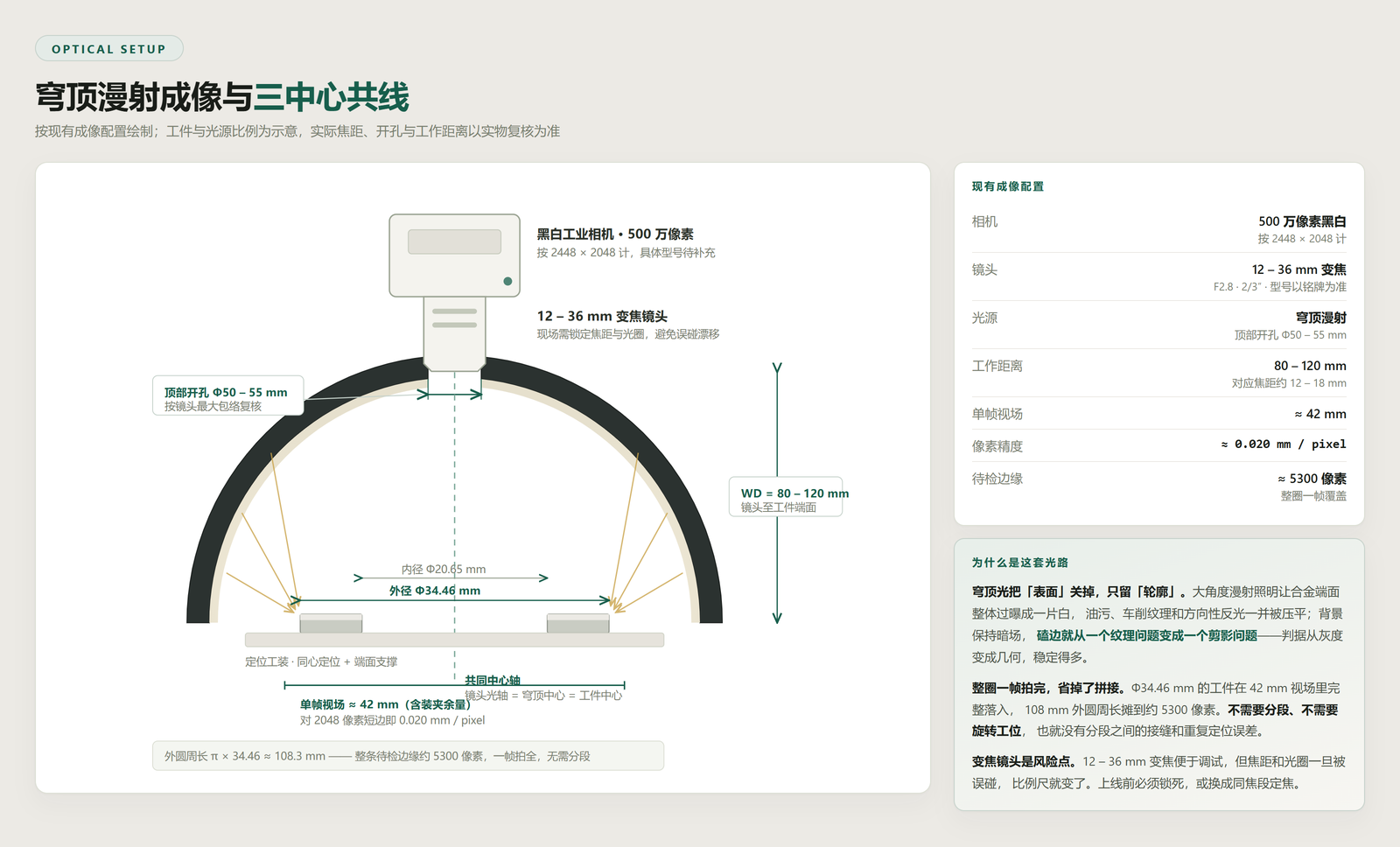
Two numbers follow. First, the circumference π × 34.46 ≈ 108.3 mm spreads over about 5300 pixels at 0.020 mm/pixel—the entire inspected edge fits in one frame, with no segmented capture and no rotary stage. That is a structural difference from large-format inspection: no segments means no seams between them, no repeat-positioning error and no dozens of exposures in the cycle. Second, a notch 0.45 mm along the arc and 0.23 mm deep occupies roughly 22 × 11 pixels at full resolution—enough for segmentation to track the contour, but not generous, which is why this sampling line is a hard constraint rather than headroom.
The dome light deserves its own note. Wide-angle diffuse illumination drives the alloy face to uniform white, flattening oil film, turning marks and directional glare together, while the background stays dark—so the outer edge becomes a high-contrast black-and-white boundary. This changes the nature of the problem: a chip is no longer a texture anomaly on a surface but a missing piece of a silhouette. Geometric criteria are far more stable than textural ones, and they map directly onto drawing tolerance.
The zoom lens is the one risk in this configuration. A 12 – 36 mm zoom is convenient during setup, but if focal length or aperture is knocked, the scale changes and every millimetre criterion silently goes with it. It must be locked before production, or replaced by a fixed focal length in the same range. The exact lens model is to be confirmed from the nameplate.
04/10Datum & Fixture
Three-centre alignment governs lighting, not centring
“Lens axis = dome centre = part centre” is the basic requirement of this optical path. Taken apart, however, the three deviations behave very differently, and the fixture only has to control one of them.
Lateral offset is absorbed in software. When the part sits off-axis, a circle parallel to the sensor still projects as a circle; only its position moves. The datum circle is fitted from the frame itself, so its centre travels with the part and the radius curve is unaffected. In several of the frames behind Fig. 01 and Fig. 03 the ring is in fact not centred, and the measurement still holds. What offset does consume is field margin—shift too far and the rim is clipped by the frame.
Height variation is absorbed the same way. A change in face height changes magnification: at 100 mm working distance, 1 mm of height is about 1 % of scale, which on the radius is of the order of 0.17 mm—larger than any chip in the table. But as long as the criterion is defined as radial intrusion relative to this frame's fitted circle, a uniform scale change cancels out. Define it instead as an absolute diameter and that 0.17 mm lands straight on the result. The form of the criterion, not the hardware, is what makes the difference.
Only face tilt has to be held mechanically. With the face tilted by α relative to the optical axis, the outer circle projects as an ellipse whose major and minor axes differ by roughly D(1 − cos α). With D = 34.46 mm:
| Face tilt | Ellipticity (axis difference) | Relative to chips |
|---|---|---|
| 2° | 0.010 mm | below baseline jitter, negligible |
| 3° | 0.024 mm | same order as baseline jitter |
| 5° | 0.066 mm | already exceeds the shallowest chip (0.05 mm) |
| 8° | 0.168 mm | approaching the deepest chip (0.24 mm) |
The fixture's key specification is therefore face tilt rather than concentricity, and holding it within 3° is a safe target. If that proves mechanically hard there is a fallback: ellipticity is a slowly varying second harmonic around the rim while a chip is a local spike, so the two look nothing alike on the unwrapped curve and an ellipse fit—or simply removing the low-order harmonics—can suppress it. That is margin, though, and should not be the first line of defence.
So what does three-centre alignment actually protect? The symmetry of the illumination. A dome's brightness distribution is symmetric about its own axis, so once the part is off-centre the incidence conditions differ around the rim, the width of the bright-to-dark transition drifts with azimuth, and the effective binarisation threshold drifts with it. That error cannot be corrected downstream. The existing material supports this: the frame with the most uneven rim brightness, where turning marks show through at the lower edge (sample F), also carries the highest baseline jitter in the set at 0.027 mm—about twice that of the cleanest frame (sample E, 0.013 mm).
Geometric centring can be recovered in software; lighting symmetry cannot. The fixture's acceptance criteria should read as face tilt and illumination uniformity, not as a vague “seat it straight”.
05/10Unwrapped Rim
Unroll the circle into a line
That a chip can sit anywhere on the rim looks like a nuisance, but it has a clean answer: fit the outer circle to establish centre and datum radius, sample the contour radius angle by angle, and unroll the whole rim into a single r(θ) curve. Once unwrapped, positional randomness disappears—the entire circumference shares one criterion, and a chip shows up as a dip in the curve.
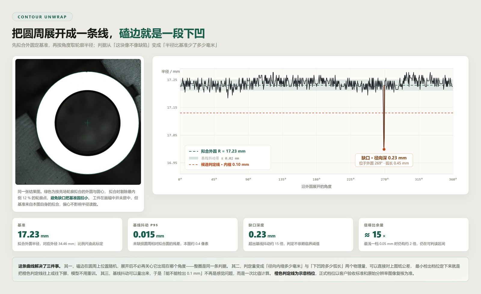
r(θ) curve of the same frame: the green dashed line is the fitted radius of 17.23 mm, the pale green band is the measured ± 0.02 mm baseline jitter, and the orange dashed line is an illustrative grade at 0.10 mm of intrusion. The dip at 269° is the chip that was boxed.The curve settles three things at once. First, the verdict becomes a physical quantity: so many millimetres of radial intrusion over so much arc, both of which map straight onto drawing tolerance, with no need to explain what a model confidence of 0.87 means. Second, signal-to-noise becomes computable—the P95 residual of the intact rim is the noise floor of this optical path, about 0.015 mm here against a 0.23 mm chip, a ratio of roughly fifteen; even the shallowest chip at 0.05 mm keeps about twice the margin. “Can it detect 0.1 mm” stops being a matter of impression and becomes one division. Third, the grade is adjustable: fixing the minimum detectable size simply moves the orange line up or down, with the model untouched.
None of this replaces the segmentation model. The unwrap supplies a stable measurement frame; the model decides which stretch of the rim actually belongs to a chip against a busy background—separating burrs, clamping marks and fixture occlusion from genuine knocks. Criterion and perception divide the work; they are not substitutes.
06/10Both Faces
One camera with a flip, or two cameras in parallel
One exposure sees one face, so two exposures per part are unavoidable. With cycle time and budget both open, two configurations stay on the table: option A uses one camera, lens and dome to shoot the faces in turn with a flip in between; option B uses two optical paths and images both faces at once, eliminating the flip.
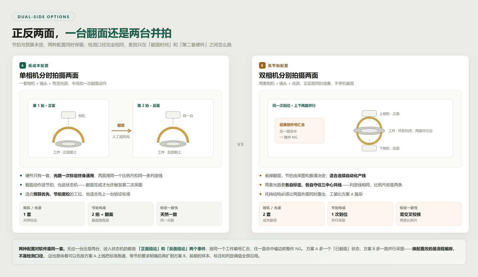
The point worth making is that the two configurations are the same system in software. One camera or two, what reaches the state machine is a front-face verdict and a back-face verdict, merged under one part ID, with a chip on either face condemning the whole part. Option A adds a “flipped” state; option B adds a parallel capture branch. Changing configuration changes the orchestration, not the inspection criteria.
That opens a practical path: start on option A, settle the minimum detectable grade, the sample library and the thresholds, then scale to option B once cycle time is fixed. Samples, labels and thresholds all carry over; only the second optical path needs new calibration.
07/10Tensor Flow
Two branches into one workflow
The vision agent runs at the edge: configuration, inference, display and output all live in one piece of software, orchestrated by dragging nodes out of an operator library and wiring them along the data flow. This project's graph is short—one branch per face: capture, pre-processing (outer-circle location and polar unwrap), semantic segmentation, event detection; the two event streams merge into one state machine, followed by image archiving and a serial device.
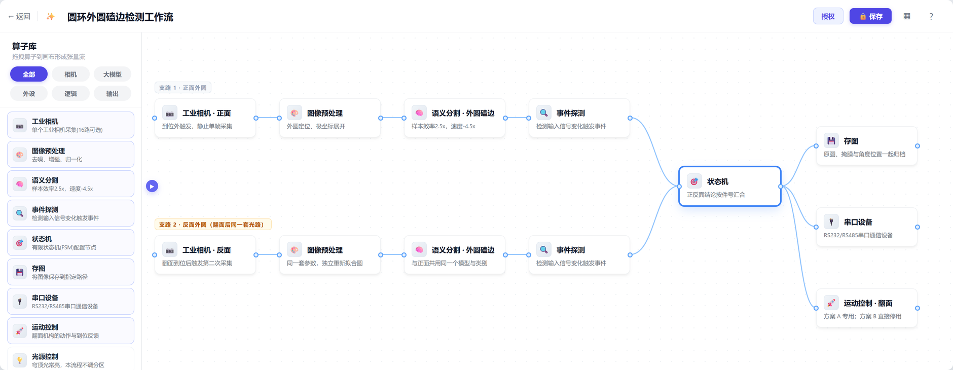
Double-clicking a node opens its sub-editor: semantic segmentation to the annotation tool, event detection to the GPU event orchestrator, state machine to the state diagram editor. The structure of this graph is independent of part geometry; moving to another ring means new calibration values, samples and thresholds, while the graph itself is reused as-is on comparable stations.
08/10Segmentation
Pixel masks, with 1–10 samples per new morphology
Chip boundaries are irregular—a sharp V in one part, a long shallow scallop in another—so box regression fits them poorly, while the downstream depth and arc conversion depends entirely on contour accuracy. The plan therefore uses pixel-level semantic segmentation: a single class, “outer-edge chip”, defined in the annotation tool from a handful of field images, with the product side starting from 1–10 sample images and minutes of setup and the mask converted to millimetres afterwards.

Having only one class actually clarifies the sampling strategy: what needs collecting is not more defect types but a sample spread that covers the detection boundary—obvious chips, borderline chips, sound parts, and the confusers that invite false calls (clamping marks, burrs, oil residue, fixture occlusion). Borderline samples matter most, since they decide where the minimum detectable grade can sit without either missing parts or crying wolf. Training and inference both run locally on the edge GPU, so station imagery stays on site.
09/10Events & FSM
From mask to “deeper than 0.10 mm”, then to one verdict per part
Segmentation only sees pixels; the line needs decidable events. Events are assembled in the GPU event orchestrator: an “object present” primitive confirms the mask lies in the rim band, a “width” primitive takes the radial intrusion against the fitted circle and compares it with a millimetre threshold, and the two meet at an AND. Arc length is a second quantity read off the same mask and becomes its own event; chip count becomes a third.
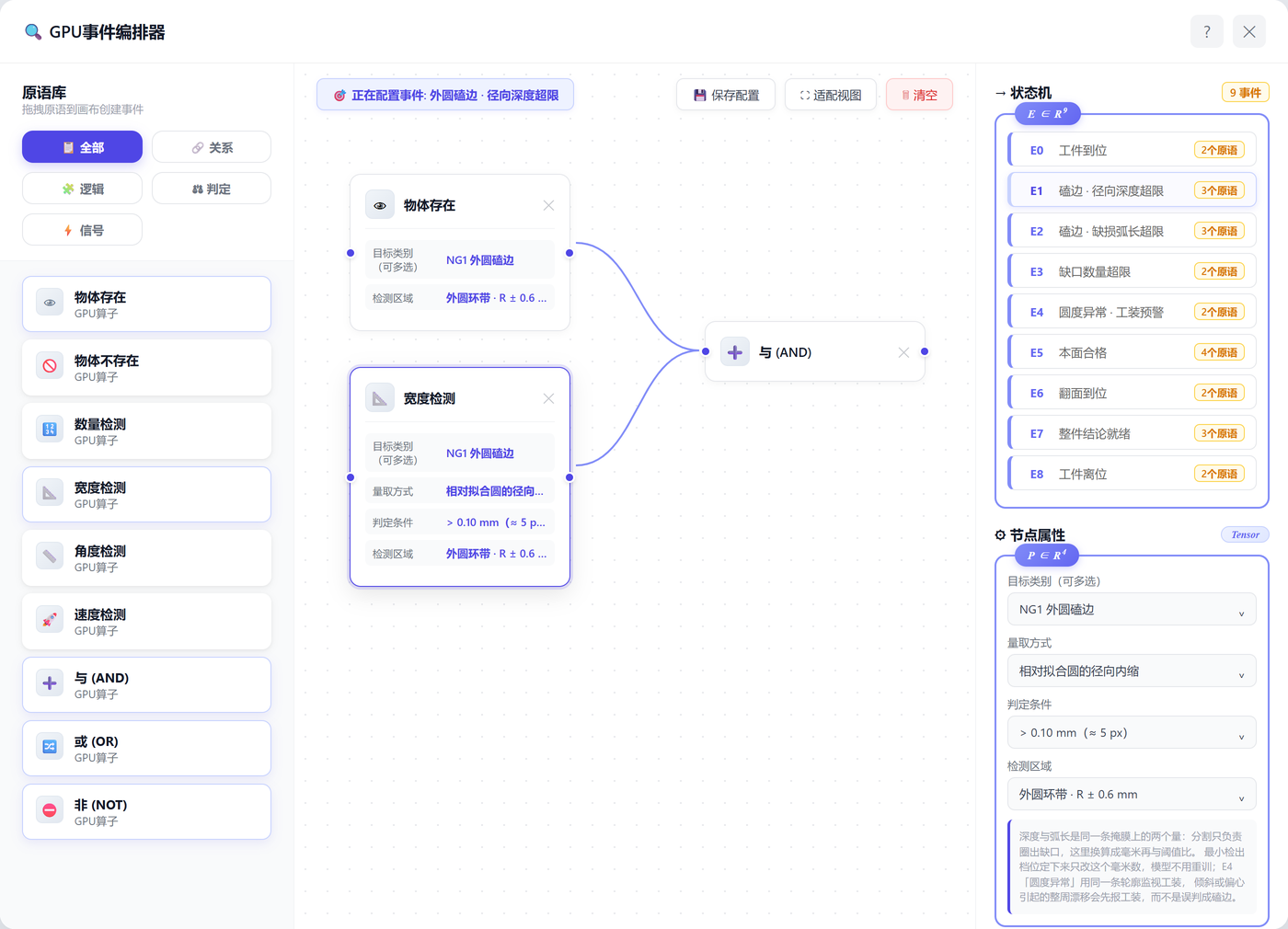
E4 watches roundness on the same contour—slow ellipticity around the rim raises a fixture alert instead of being mistaken for a chip.Keeping thresholds at the event layer rather than inside the model is the pivot of this structure, and it matters more than usual here because the minimum detectable grade has not been set yet. The system can go live on an initial grade and start producing data; when the customer's standard arrives, what changes is a millimetre value in the recipe, with samples, labels and model untouched. The same holds for the allowed arc length and the permitted chip count per part.
The state machine then assembles these events into the station's flow. A part arrives and enters front-face inspection; only a passing front face triggers the flip and back-face inspection; only two passing faces release the part and increment the count. A hit on either face turns NG, and the archive records angular position, radial depth and arc length together. One cycle-time detail is worth flagging: a part already condemned on the front face is not flipped—it is settled immediately, and flipping only ever happens on parts that passed.
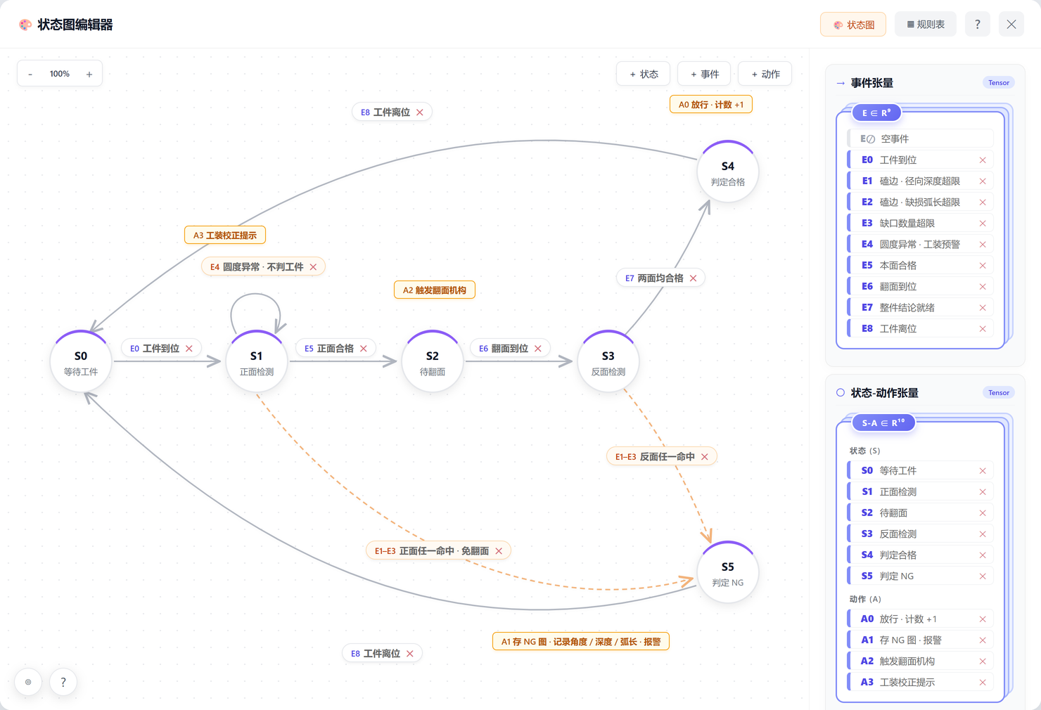
E1–E3 on the front face take the dashed path straight to S5, skipping the flip; E4 roundness anomaly does not judge the part at all but loops back to S1 with a fixture-correction prompt, keeping a clamping problem out of the reject rate.What the machine returns is not “does this frame look wrong” but “may this part pass under the current recipe”—with an angle, a millimetre value and a reviewable record.
10Deployment
Edge-local inference: collect the data, then set the standard
The system sits on five layers: camera and dome light capture; gigabit industrial Ethernet moves frames inside the plant network only; an edge GPU runs segmentation, size conversion, event decisions and state transitions; the front end offers live view, NG alarms, manual review and retrieval by time, part ID or angle; and a recipe layer holds camera parameters, calibration values, model versions and thresholds together. Raw frames, masks, result images and verdicts are archived per part—both as traceability material and as the sample source for the next round of tuning.
For a project whose standard is still open, that archive carries extra value: once the system runs, every part's depth and arc length is recorded, and within a few weeks there is a real size distribution. The minimum detectable grade can then be set on data rather than on impression.
System hardware
The table fixes equipment categories and configuration direction only; exact models are frozen after physical verification and once cycle time is known.
| # | Equipment | Configuration direction | Purpose |
|---|---|---|---|
| 1 | Industrial camera | 5 MP monochrome, external trigger | Capture both faces of the rim at ≈ 0.020 mm/pixel |
| 2 | Industrial lens | 12 – 36 mm zoom, locked or replaced by a prime before production | Match the ≈ 42 mm frame at 80 – 120 mm working distance |
| 3 | Dome light | Top aperture re-checked against the lens envelope, Φ50 – 55 mm to start | Wide-angle diffusion to flatten oil film and directional glare |
| 4 | Locating fixture | Concentric seat with face support, face tilt held within 3° | Preserve illumination symmetry and repeatable placement |
| 5 | Flip mechanism / second path | Selected per option A or option B | Cover the back face of the rim |
| 6 | Position sensor / PLC interface | Industrial digital I/O or fieldbus | Trigger capture, receive OK/NG, gate the station |
| 7 | Edge computing unit | Sized for two-face inference per part plus storage | Segmentation, size conversion, UI and archiving |
| 8 | HMI and alarm | Industrial monitor, tri-colour tower light, buzzer | Display, alarm, review and operation on site |
Rollout sequence
One step departs from the usual order: standard alignment comes before sample collection. Labelling against an undefined criterion means the labelling convention is reworked along with the criterion.
| Stage | Duration | Main work | Deliverable |
|---|---|---|---|
| Standard alignment | 1 week | Fix the minimum detectable grade, allowed loss, dual-face verdict rule and review policy | Acceptance criteria · labelling convention |
| Imaging freeze | 1 week | Lock focal length, aperture and exposure; verify fixture concentricity and tilt; calibrate mm/pixel on a reference part | Calibration record · fixture acceptance items |
| Samples and labels | 1–2 weeks | Collect sound, obvious, borderline and confuser samples; label to one convention | Sample library · label consistency check |
| Pilot deployment | 1–2 weeks | Commission recipes, event thresholds and the state machine; merge dual-face verdicts and connect the PLC | Live system · configuration record |
| Trial run and tuning | 2 weeks | Adjust thresholds and model on false-call and escape samples; set the grade from the measured distribution | Tuning report · size distribution · O&M manual |
The boundaries are worth stating. This plan addresses contour-type defects—knocks that remove material from the outer silhouette. If acceptance also covers texture-type defects such as face scratches, pitting or discolouration, blowing the face to white with a dome no longer works and a second recipe with low-angle or ring lighting is required, which is a different technical route. Part height is still unconfirmed and affects both depth of field and fixture design; the lens model and outer diameter must be verified physically, with the dome aperture following from that. All measurements quoted here come from downsampled result images and are used to establish orders of magnitude; the minimum detectable grade and the OK/NG boundary follow full-resolution imagery and the customer's acceptance standard.
Blue
Industrial vision algorithm engineer · author
Computer vision background, working on the engineering side of optical imaging and defect segmentation. Prefers to freeze lighting and sampling resolution before discussing models; in recent years mainly replacing per-class AOI tuning with few-shot vision foundation models. Has worked on inspection and SOP process-monitoring deployments for consumer-electronics parts, appliance hardware, lithium battery and automotive components, and owns field calibration, recipe management and post-launch iteration.