Vision LLM · Appearance QC / Field Plan
Food Packaging: Six-Side Appearance Inspection for Milk Powder Scoops — Field Plan
One scoop, six faces, dirt cracks and short shots— a six-camera surround station captures every face in a single cycle, and turns "does it look like a defect" into a millimetre number you can edit in the recipe.
Key takeaways
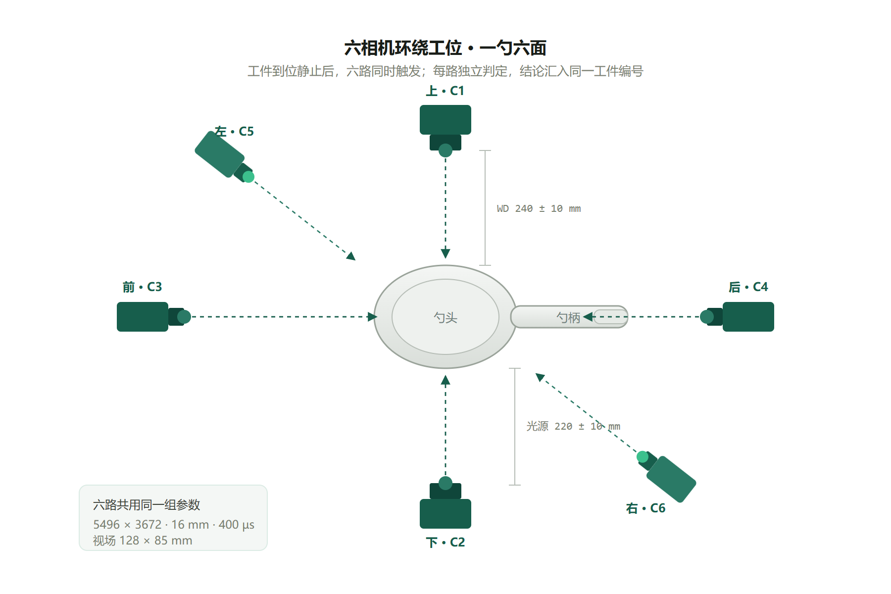
- Six faces is not six shots—it is one frame. Six cameras surround a single station; once the part is seated and still, all six trigger together. One cycle covers all six faces, with no flipping, no segmentation and no re-positioning.
- Freeze the sampling line first. 5496 × 3672 over a 128 × 85 mm field gives about 0.023 mm/pixel; a 0.1 mm dirt spot covers about 4 pixels, a 0.5 mm crack about 22 pixels. Whether a class is detectable becomes a calculation, not a guess.
- 400 µs simultaneous exposure suppresses reflection. The scoop is an injection-moulded part with directional reflectance; short exposure plus a black background suppresses ambient light and specular glare, widening the grey-level gap between defect and normal surface.
- Thresholds live in the recipe, not in the model. Dirt area, crack length and short-shot size are all millimetre numbers in the event layer; when the acceptance standard changes, only the number changes—the model is not retrained. A new defect class starts from 1–10 sample images and minutes of setup, with inference running locally on an edge GPU.
A milk powder scoop is the standard measure inside every can: injection-moulded, with a glossy finish, but incoming material and the moulding process bring appearance defects—dirt, cracks, short shots, deformation. These parts are small, low-value and high-volume, and appearance QC has long relied on human eyes: six faces flipped and inspected piece by piece, with miss rates climbing as fatigue sets in; defective images and verdicts are rarely recorded in a structured way, so traceability depends on memory. This plan is not about "whether there is a model"—it is about folding six-side appearance inspection into a configurable, reviewable and replicable inspection standard.
01/09Challenge
Too many faces, defects too small
The defect list for a milk powder scoop is short: dirt, cracks, short shots, deformation, plus the usual injection-moulding flash and sink marks. The difficulty lies in three additional conditions. First, all six faces must be inspected—inside and outside the bowl, front and back of the handle, both side edges; a miss on any face flows straight to the consumer. Second, the defects are small and morphologically similar: a 0.1 mm dirt spot is nearly indistinguishable from normal moulding texture under ordinary lighting. Third, the part is a reflective injection-moulded piece: when ambient light changes, the image of the same part changes with it, and classical thresholding simply cannot hold.
What makes it harder is the elasticity of the standard. "How small a dirt spot counts as NG" often has different answers for different customers and different batches. The classical AOI approach is to collect samples against an assumed grade, train a model and tune thresholds, then redo the whole cycle once the standard is clarified—the rework often costs more than the first round. So this plan treats the minimum detectable grade as a parameter to be filled in, not as a known condition.
What six-side appearance inspection must deliver is not an accuracy figure, but a quantifiable detection floor—and the ability to change a single number when the standard moves.
02/09Six-Side Coverage
Six cameras around one station, all faces in one shot
The intuitive way to inspect six faces is one camera plus a flipping mechanism, six exposures. But flipping means re-positioning, and six exposures mean six times the cycle time—on a line where the beat is measured in seconds. The plan therefore uses a six-camera surround station: one each for top, bottom, front, back, left and right. Once the part is seated and still, all six trigger together; one cycle covers all six faces.
The key to this layout is not the camera count but the mutual relationship of the optical axes. Top and bottom are opposed vertically, covering the inner bowl and the back of the handle; front and back are opposed horizontally, covering the bowl tip and the handle tail; left and right sit at a 30° angle to catch the side edges and bowl walls. There is no mechanical motion between the six paths, so there is no re-positioning error; each path leaves fixture clearance in its field, so minor part offsets do not cut an edge out of frame.
It is worth noting that the six paths are the same software. Whether six cameras or one camera shooting six times, what enters the state machine is six verdicts merged under the same part ID—any face hit makes the whole part NG. Six cameras simply compress "six times" into "once"; the inspection standard does not change.
03/09Sampling
0.023 mm/pixel: how many pixels does a defect occupy
Sampling resolution has to be settled first. The current configuration is a 20-megapixel colour camera, a 16 mm fixed-focus lens and a white ring light, at 240 mm working distance, giving a 128 × 85 mm field. From 5496 × 3672, 128 mm across 5496 pixels is about 0.023 mm/pixel; 85 mm across 3672 pixels is about 0.023 mm/pixel—consistent in both directions.
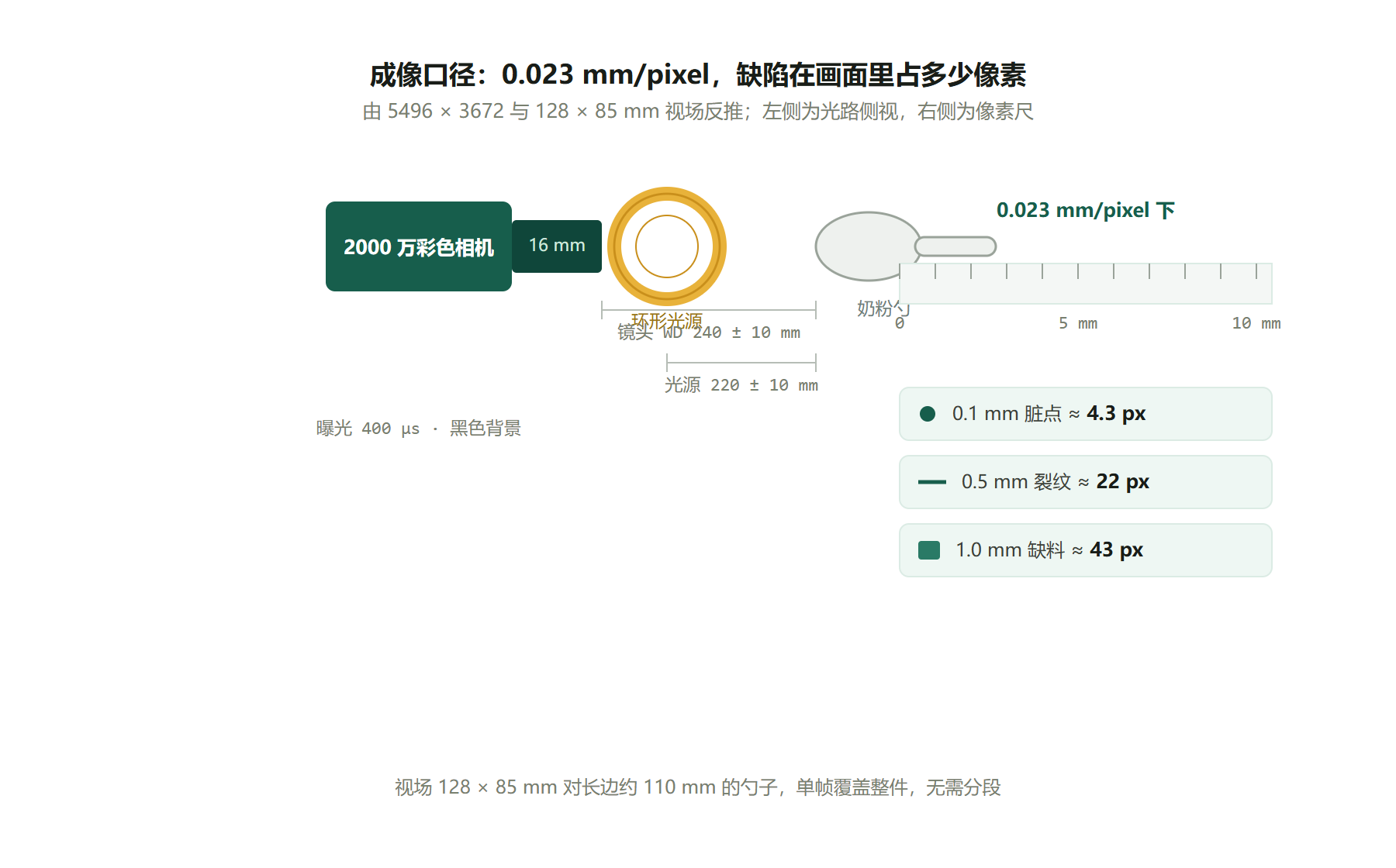
Three numbers follow. First, the scoop's long edge is about 110 mm; a 128 mm field with fixture clearance covers the whole part in one frame—no segmentation needed. Second, a 0.1 mm dirt spot covers about 4.3 pixels, already near the floor of pixel-level segmentation; a 0.5 mm crack covers about 22 pixels and a 1.0 mm short shot about 43 pixels—both enough for a mask to hug the contour. Third, 400 µs short exposure plus a black background suppresses ambient light and the directional reflectance of the moulded surface, widening the grey-level gap between defect and normal—this is the precondition for stable segmentation downstream.
The ring light sits closer than the lens (220 mm versus 240 mm) to steepen the incidence angle and shrink the shadow zone inside the bowl. Light stability is the only variable that must be held on site: the moulded surface is highly reflective, and a 5 % drift in brightness can push the grey level of the same spot out of the threshold band. That is why the notes explicitly require "stable lighting, with some shading from ambient light"—this is not a nice-to-have, it is a hard constraint.
04/09Defect Samples
Real shots from six faces: what the defects look like
The following six frames were captured by the six cameras in a single cycle, cropped by face. Dirt on the inner bowl appears as an irregular dark patch; a crack on the handle front appears as a fine line; a short shot on an edge appears as a local contour recession. The three classes look very different in the image—which is exactly why they must become separate events sharing the same segmentation base.
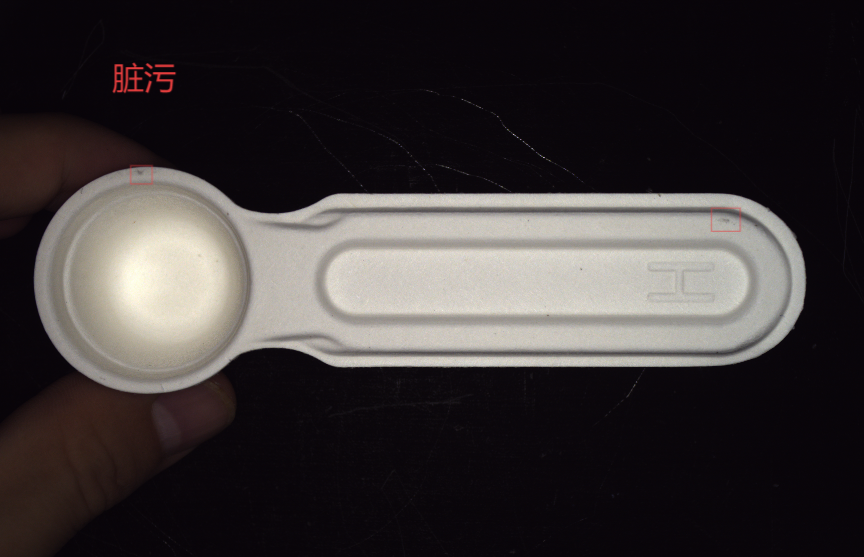
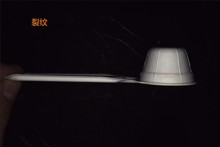

It should be noted that these frames are outputs from the lighting-trial stage: exposure and background are already frozen to the production standard, but the defect sample count is not yet enough to cover every morphology. Before go-live, the sample spectrum must be filled in across four categories—normal, obvious defect, borderline defect and distractor. Borderline samples are especially critical: they directly determine where the minimum detectable grade can be set without either missing defects or over-reporting.
05/09Tensor Flow
Six branches into one workflow
The vision agent runs on the edge: configuration, inference, HMI and outputs share one software stack, wired zero-code on a canvas—drag operators from the library, connect them by data flow. The flow for this project is regular: after triggering, six branches capture in parallel; each branch pre-processes (locate and normalise), runs semantic segmentation, then event detection; the six event streams merge into one state machine, followed by archiving and host communication.
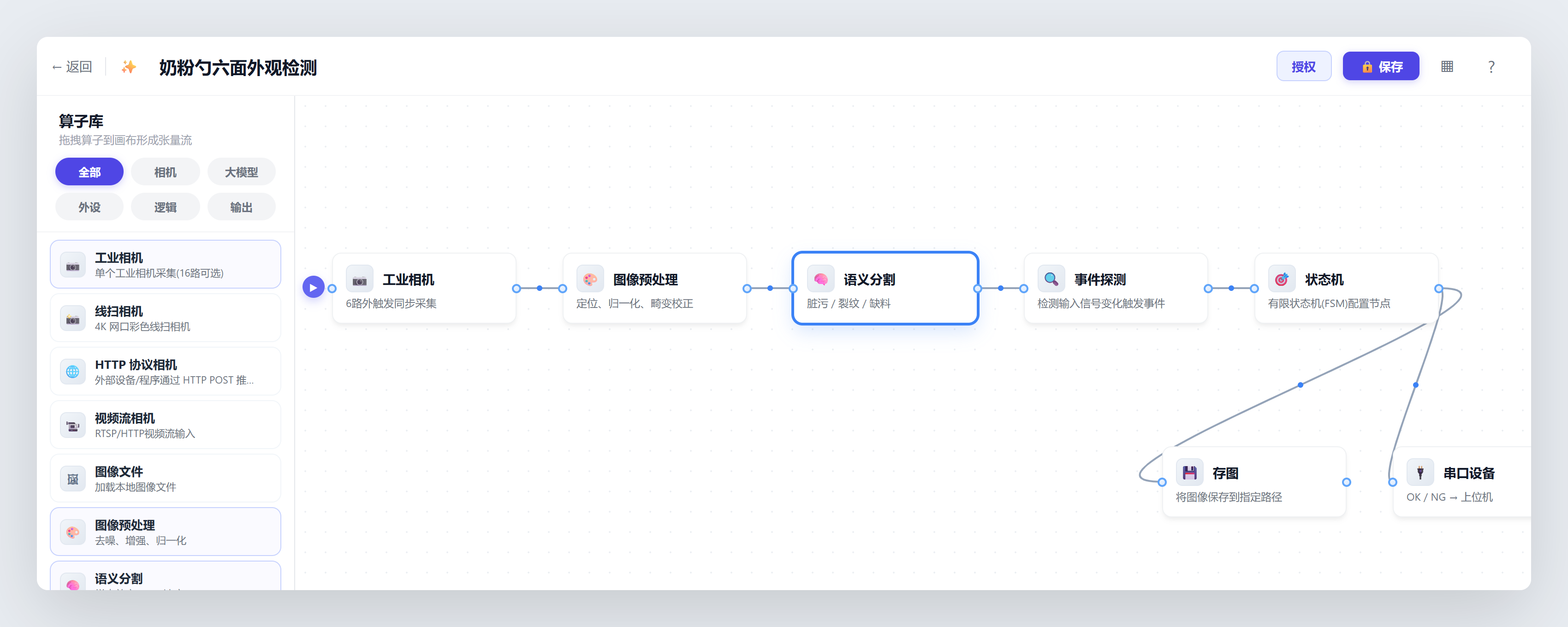
The structure of this flow is independent of product specification: a different scoop shape only changes calibration values, samples and thresholds, and the flow itself can be reused on similar stations. Six parallel branches do not demand much from the edge GPU: one 5496 × 3672 segmentation takes about 80 ms, six in parallel about 120 ms; with event decision and state-machine transitions, total per-part time stays under 200 ms—well below the line beat.
06/09Segmentation
Pixel masks: lock a new morphology with 1–10 samples
Scoop defects rarely have regular boundaries: dirt is an arbitrary blob, a crack is a fine broken line, a short shot is a gradual contour recession. Boxes fit these poorly, and the downstream size decision depends entirely on contour accuracy. The plan therefore uses pixel-level semantic segmentation: define the three classes "dirt", "crack" and "short shot" in the annotation tool with a small number of field images, starting from 1–10 sample images and minutes of setup on the product side, then compute area, length or maximum enclosing size from the output mask.
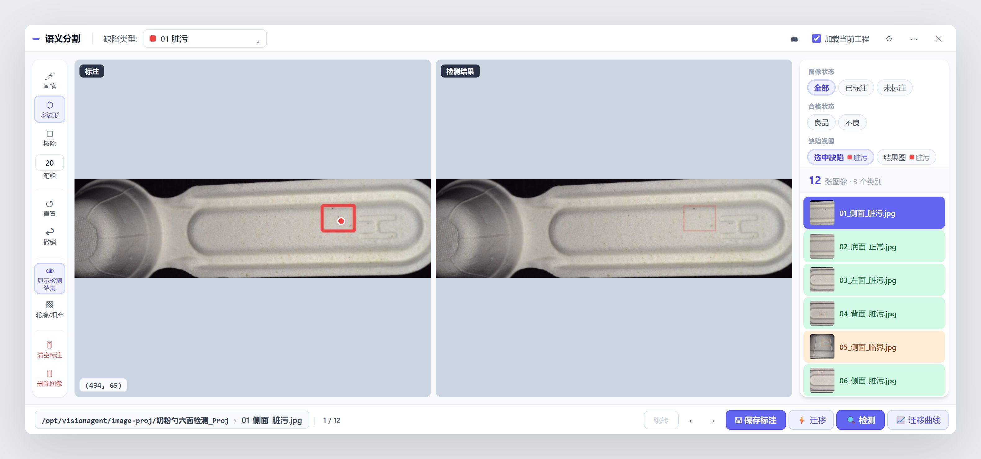
This is what makes "six-side appearance inspection" affordable. A few-shot base means adding a class does not restart a collection-and-long-training cycle: between batches or between colours of the same scoop, morphologically similar classes often transfer with only a small amount of additional annotation. Training and inference both run locally on the edge GPU, so station frames never leave the plant—good for both real-time performance and data security.
07/09Events
Turning a mask into "dirt over 0.5 mm²"
Segmentation only sees pixels; the line needs decidable events. Events are composed in the GPU event composer: "object presence" confirms the mask hits the target class, then "area detection" or "length detection" compares the mask size against a millimetre threshold, and the two are joined with AND. The dirt grade lands here—first "object presence" confirms the mask hits the dirt class, then "area detection" compares the mask area against a square-millimetre threshold.
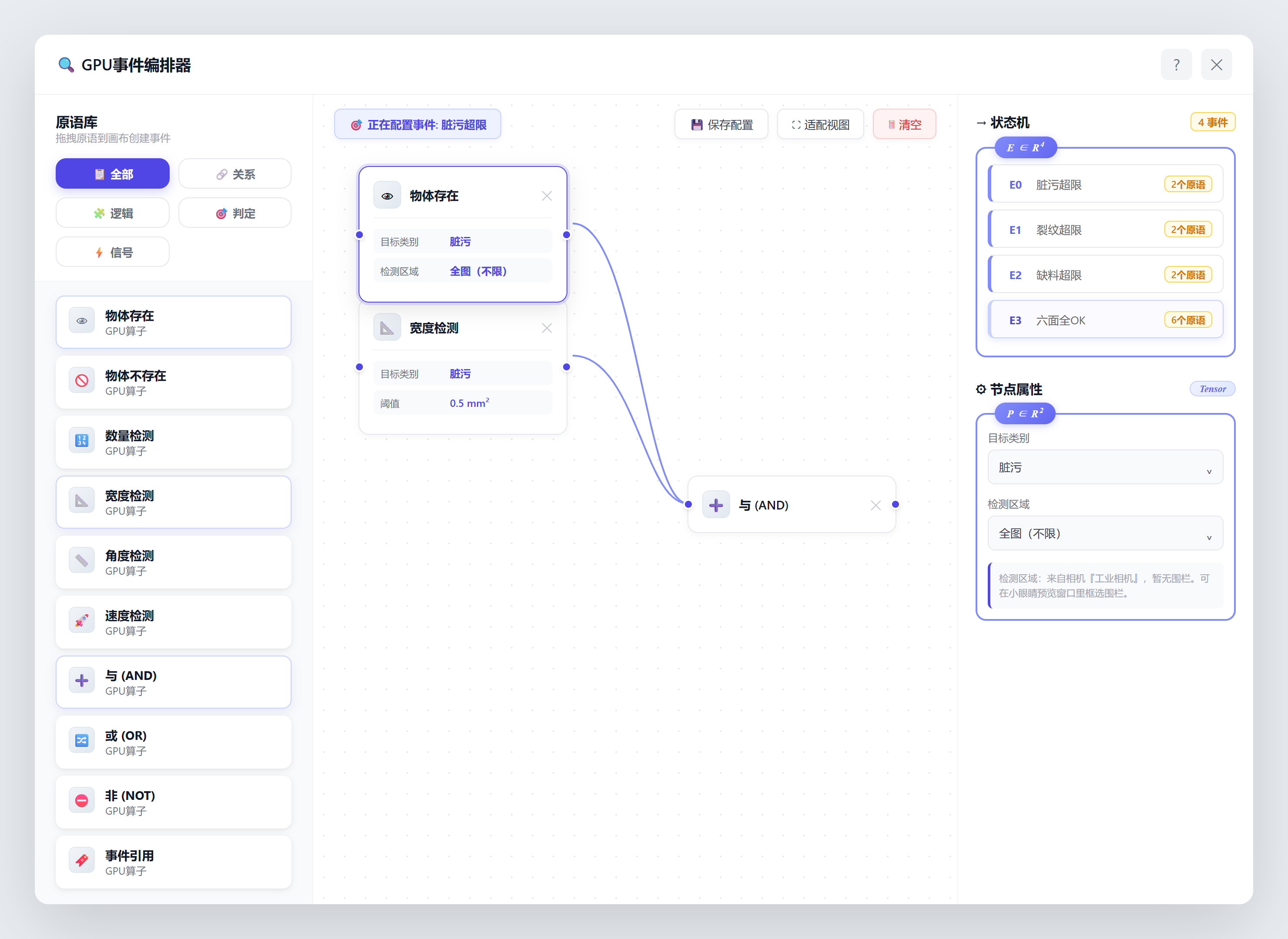
Keeping thresholds in the event layer rather than inside the model is the structural point. The 0.3 mm² and 0.5 mm² grades share one mask and one model, so changing the acceptance grade is a single number; likewise, the upper limit on crack length and the tolerance on short-shot depth are all numbers in the recipe, with the perception layer untouched. This matters especially on lines where tolerance grades change frequently.
08/09State Machine
Release only when all six faces are clear
Six-path decision creates a problem manual inspection never had: one part yields six verdicts, and something has to fold them into a single conclusion. The state machine weaves discrete events into the field process: once the part is seated, it enters six-face capture; only when all six paths pass does it release and count; any face hit sends it to NG, with the face, class and size recorded in the archive. NG parts leave the station for review, and can be re-seated and re-inspected after a passing re-judgement.
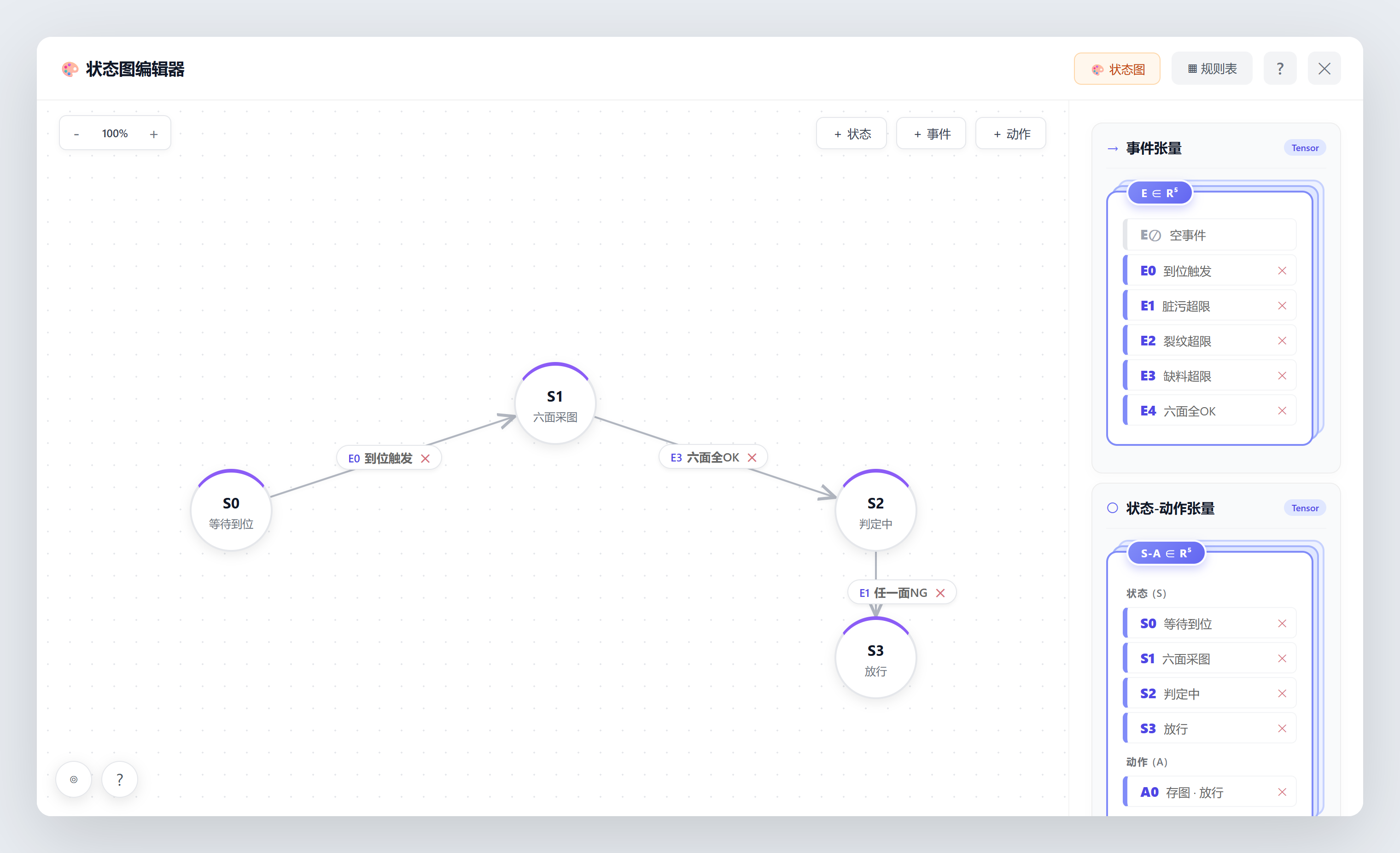
The machine does not answer "does this frame look like a defect" but "may this part pass under the current recipe"—with the face, the class, the millimetres and a reviewable record attached.
09Deployment
Edge-local inference, with samples and verdicts accumulating together
The system sits on five layers. Six cameras and ring lights capture; a gigabit industrial network keeps traffic inside the plant, so images never leave the site; the edge GPU runs segmentation inference, event decision and state-machine transitions; the front end provides live view, NG alarm, manual review and traceability searchable by time, part ID and face; the recipe manager unifies camera parameters, calibration values, model versions and thresholds. Original images, masks, result images and verdicts are archived per part—both traceability material and the sample source for the next round of optimisation.
For a project whose standard is not yet locked, archiving has an extra value: once the system is running, the defect size distribution of every part is recorded, and within a few weeks there is a real size distribution. The minimum detectable grade can be set on data, not on feeling.
Hardware configuration
The table fixes categories and configuration direction only; specific models freeze after physical review and cycle-time confirmation.
| # | Device | Configuration direction | Purpose |
|---|---|---|---|
| 1 | Industrial camera | 20 MP colour, external trigger | Six-path capture, ≈ 0.023 mm/pixel |
| 2 | Industrial lens | 16 mm fixed focus | Matches 128 × 85 mm single-frame field, WD 240 mm |
| 3 | Ring light | White ring, 220 mm working distance | Steep incidence to suppress reflection, black background to absorb stray light |
| 4 | Light controller | 4-channel × 2 | Independent triggering and brightness management for six lights |
| 5 | Positioning fixture | Six-face locating + black background | Holds repeatability and imaging consistency |
| 6 | Presence sensor / PLC interface | Industrial digital I/O or communication interface | Triggers capture, receives OK/NG, controls pass-through |
| 7 | Edge computing unit | Sufficient for six-path parallel inference and data storage | Segmentation inference, event decision, HMI and archiving |
| 8 | HMI and audible/visual alarm | Industrial display, stack light, buzzer | On-site display, alarm, review and operation |
Rollout
One step is ordered differently from usual: standard alignment comes before sample collection. If annotation starts before the criterion is set, the annotation spec is reworked together with the criterion.
| Stage | Duration | Main work | Deliverables |
|---|---|---|---|
| Standard alignment | 1 week | Define minimum detectable grade, allowed range and review rules for each defect class | Acceptance criteria table · annotation spec |
| Imaging freeze | 1 week | Lock exposure and light brightness, verify fixture repeatability, calibrate mm/pixel with a reference part | Imaging calibration record · fixture acceptance items |
| Samples and annotation | 1–2 weeks | Collect normal, obvious-defect, borderline-defect and distractor samples, annotate to a unified standard | Sample library · annotation consistency check |
| Pilot deployment | 1–2 weeks | Tune recipes, event thresholds and state machine, merge six-face verdicts and connect to the host | Go-live system · configuration record |
| Trial-run optimisation | 2 weeks | Adjust thresholds and model from false-positive/false-negative samples, re-set grades from the measured distribution | Optimisation report · size distribution · operations manual |
The boundary is explicit. This plan targets surface-type defects—dirt, cracks, short shots and deformation that cause visible anomalies on the six faces. If the acceptance scope also includes structural defects such as internal bubbles or weld lines, external ring-light illumination no longer applies, and a second recipe based on transmission or X-ray is needed—a different technical path. All measurements in this article are taken from lighting-trial outputs and are used to establish magnitude; the minimum detectable grade and the OK/NG boundary are subject to official samples and the customer's acceptance standard.
Blue
Industrial vision algorithm engineer · author
Computer vision background, with years of engineering work on optical imaging and defect segmentation. Believes in fixing the lighting and sampling budget before talking about models; in recent years mainly replaces per-class-tuned classical AOI with few-shot vision foundation models. Has been involved in line-side inspection and SOP process-monitoring deployments across 3C structural parts, home-appliance hardware, lithium batteries and automotive components, and also owns field calibration, recipe management and continuous iteration after go-live.