Vision LLM · Appearance QC / Field Plan
Battery Tab Appearance Inspection — Field Plan
Two materials, thirty defect names, a 1410 mm long edge— fold the names into 7 imaging families, swap incidence angle inside one 36-zone light, and let few-shot segmentation collapse 30 classes into 4 recipes.
Key takeaways
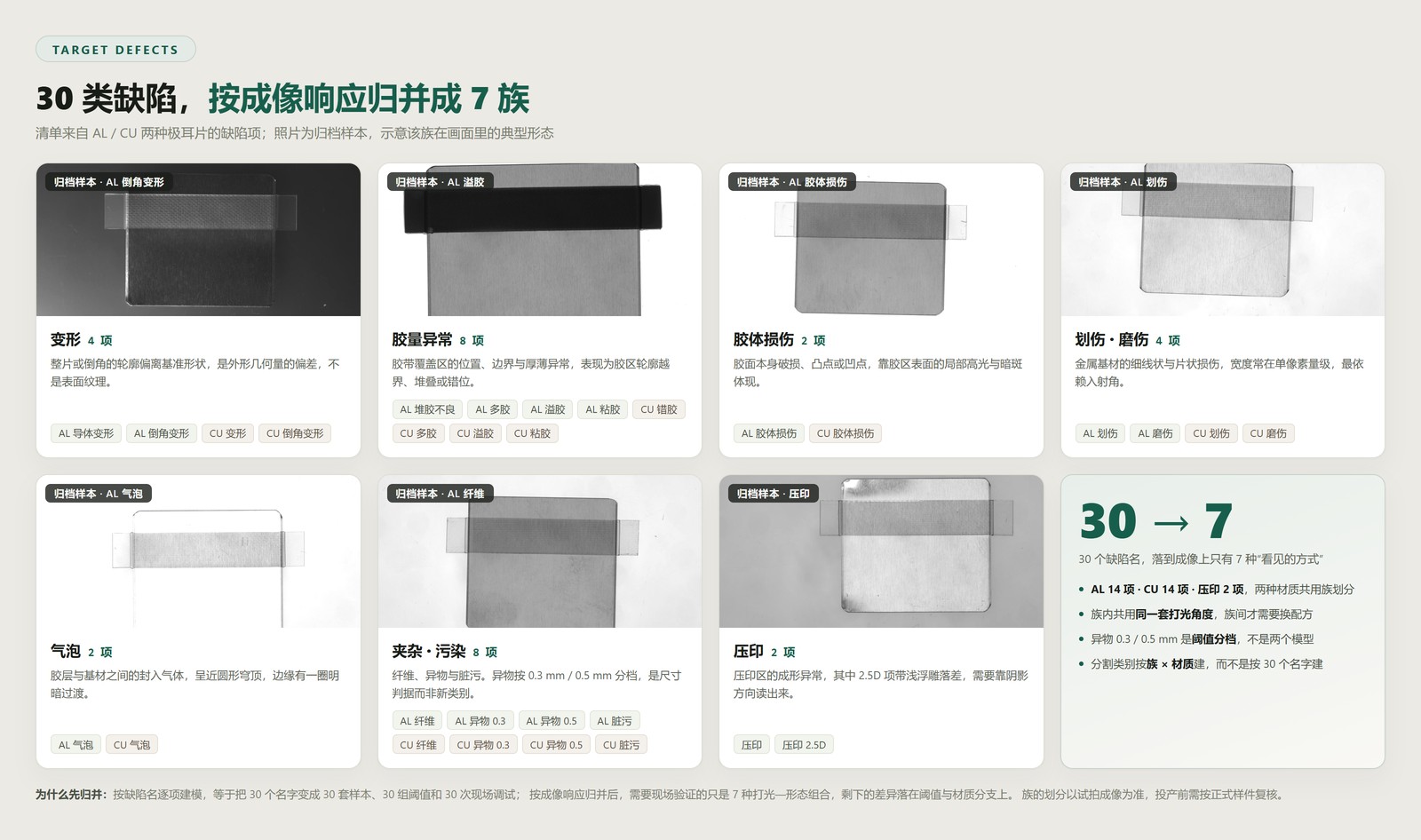
- Thirty defect names, seven ways of seeing. The list is written by material and process, but in the image there are only seven families: deformation, adhesive volume, adhesive damage, scratch/abrasion, bubble, inclusion/contamination and embossing. Lighting is shared inside a family; recipes change only across families.
- Freeze the sampling line first. 4096 × 3000 over a 68 × 52 mm field gives 0.017 mm/pixel—a 0.3 mm inclusion covers about 18 pixels. That line, not a bigger model, is what makes the smallest class detectable.
- Switching zones is switching incidence angle. A 36-zone white light already spans different radii and azimuths; lighting a different ring is an angle change. Four morphologies, four recipes—no extra camera, lens or lamp.
- The long edge must be segmented. A 68 mm frame against a 1410 mm edge means roughly 21–23 segments, each running 4 recipes: 84–92 exposures per part. Cycle time is decided here, not in inference.
- Few-shot start, edge-local run. A new defect class starts from 1–10 sample images and minutes of setup; capture, segmentation, decision and archiving all run on the edge GPU, so frames stay on site.
A battery tab is the current outlet of a cell: a metal foil carrying a strip of insulating adhesive, tens of millimetres wide and over a metre long. Appearance QC here has long relied on human eyes—defects are small, the types are many and they look alike; one shift is more than attention can hold, and an escape goes straight into the cell. Defect images and verdicts are rarely kept in structured form, so traceability falls back on memory. The problem this plan solves is not “do we have a model”, but how to collapse 30 defect names into criteria that can be configured, reviewed and replicated.
01/10Challenge
Too many defect names, too few ways to image them
The list holds 30 entries: 14 on aluminium tabs, 14 on copper tabs, 2 on embossing. The names differ widely—“adhesive pile-up” and “double adhesive (mixed sheets)” are two process causes; “inclusion 0.3 mm” and “inclusion 0.5 mm” are two quality grades. Treated the classic AOI way, 30 names mean 30 sample sets, 30 threshold groups and 30 rounds of onsite tuning, repeated whenever the material or the incoming batch changes. Training engineers stay resident, and replication never starts.
Look at it from the sensor side instead. A camera cannot see a process cause; it sees grey levels. Pile-up and double adhesive are both a raised band outside the tape boundary; 0.3 mm and 0.5 mm inclusions are two grades read off the same mask. What actually needs distinguishing is which light makes the defect appear at all. So the first step is not choosing a model—it is pushing 30 names back onto the imaging layer and counting how many genuinely different ways of seeing remain.
The defect list is written by process; the inspection plan has to be written by imaging. Every step downstream pays twice while those two vocabularies disagree.
02/10Families
Thirty into seven: shared light inside a family, new recipe across
Re-sorted by “what it looks like and what light it needs”, the list collapses into seven families. The immediate payoff: one optical path and one segmentation class set per family, with a recipe change only across families—which is how 30 rounds of tuning become the 4 lighting experiments of Section 04.
| Family | Covers | Imaging signature | Measurement |
|---|---|---|---|
| Deformation | 4 | Whole-sheet or chamfer contour departing from the reference shape | Max deviation from reference contour |
| Adhesive volume | 8 | Tape position, boundary or thickness anomalies: contour overrun, stacking or gaps | Boundary position and covered area |
| Adhesive damage | 2 | Broken or pitted adhesive surface, local highlight and dark-patch change | Damaged area and max extent |
| Scratch / abrasion | 4 | Fine linear or patch damage on the foil, often at single-pixel width | Scratch length and max width |
| Bubble | 2 | Gas trapped between adhesive and foil, near-circular dome | Equivalent diameter |
| Inclusion / contamination | 8 | Fibre, foreign matter, soiling; wide size range | Max bounding size of the mask, graded 0.3 / 0.5 mm |
| Embossing | 2 | Forming anomalies in the embossed zone; the 2.5D item adds shallow relief | Contour and depth contrast of the embossed zone |
Two notes. First, aluminium and copper are different substrates, but a family images the same way on both—copper's higher reflectance shows up as a brightness offset inside the same recipe, not as another family. Second, the 0.3 mm and 0.5 mm inclusions are not two classes but two grades on one mask: segmentation gives the contour, the event layer compares its max bounding size against a threshold. Changing the acceptance grade edits one millimetre value; the model is untouched. On lines where tolerances move often, that separation is what keeps maintenance cost flat.
03/10Sampling
0.017 mm/pixel: draw the sampling line before discussing accuracy
The smallest criterion on the list is a 0.3 mm inclusion. For it to form reliably in the image, sampling resolution has to be settled first. The imaging trial uses 0.017 mm/pixel: a 0.3 mm target spans about 18 pixels and a 0.5 mm target about 29—enough for a pixel-level mask to hug the contour, and enough to separate the two grades. Relax to 0.05 mm/pixel and 0.3 mm is down to six pixels, at which point even a strong model is only guessing.
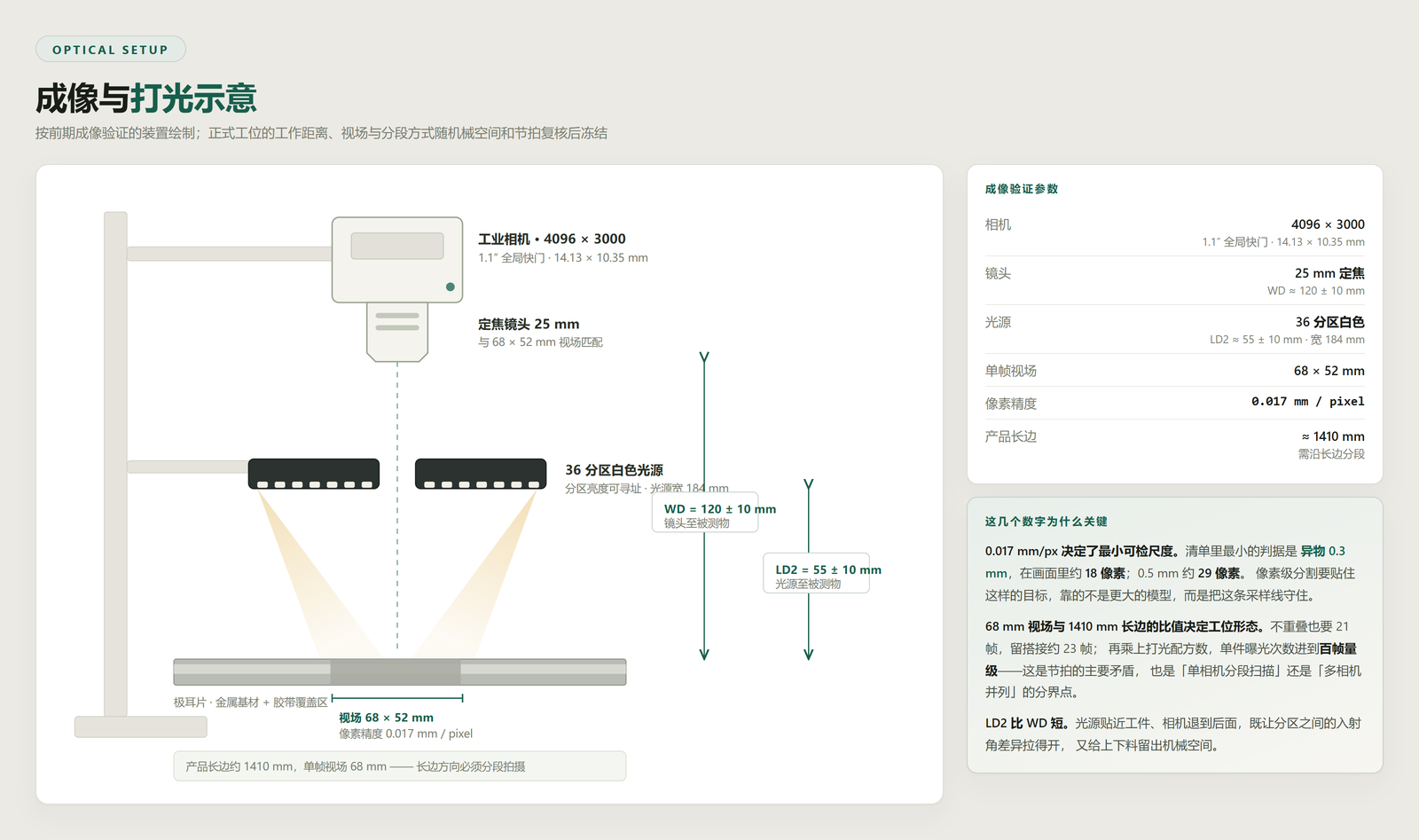
From 0.017 mm/pixel and 4096 × 3000, the single-frame field follows: 68 × 52 mm. That number then decides two things—a 25 mm fixed lens at roughly 120 mm working distance, and the fact that a 1410 mm edge has to be captured in segments, which is the station-layout problem of Section 05. The light sits closer than the camera (LD2 ≈ 55 mm) to widen the angular difference between zones while leaving mechanical room for loading.
Camera, lens and light reflect the imaging-validation stage. Exposure, working distance and station layout freeze after official samples, mechanical space and real cycle time have been checked.
04/10Zoned Light
One light: lighting a different zone is changing the incidence angle
The seven families do not ask for the same light. A scratch is a microscopic groove in the foil with no height of its own—only near-coaxial light, returning along its own path, makes the groove wall fall off the bright field and read as a dark line. A bubble is a dome under the adhesive—only grazing light leaves the bright-one-side, dark-the-other signature on a frontal view. Adhesive scratches sit between the two and want a mid-high angle from the inner rim of the sectors. Dedicating a lamp to each morphology would put four light assemblies on one station, which neither the budget nor the mechanical space supports.
A 36-zone white light removes that need. The zones already sit at different radii and azimuths, so choosing which ring and which azimuths to light is equivalent to changing the incidence angle—no camera move, no lens change, no added lamp; the switch is one recipe command. The four morphologies therefore collapse into four recipes along a single axis: the closer a defect is to pure texture, the further inward the light moves; the more three-dimensional the relief, the further outward.
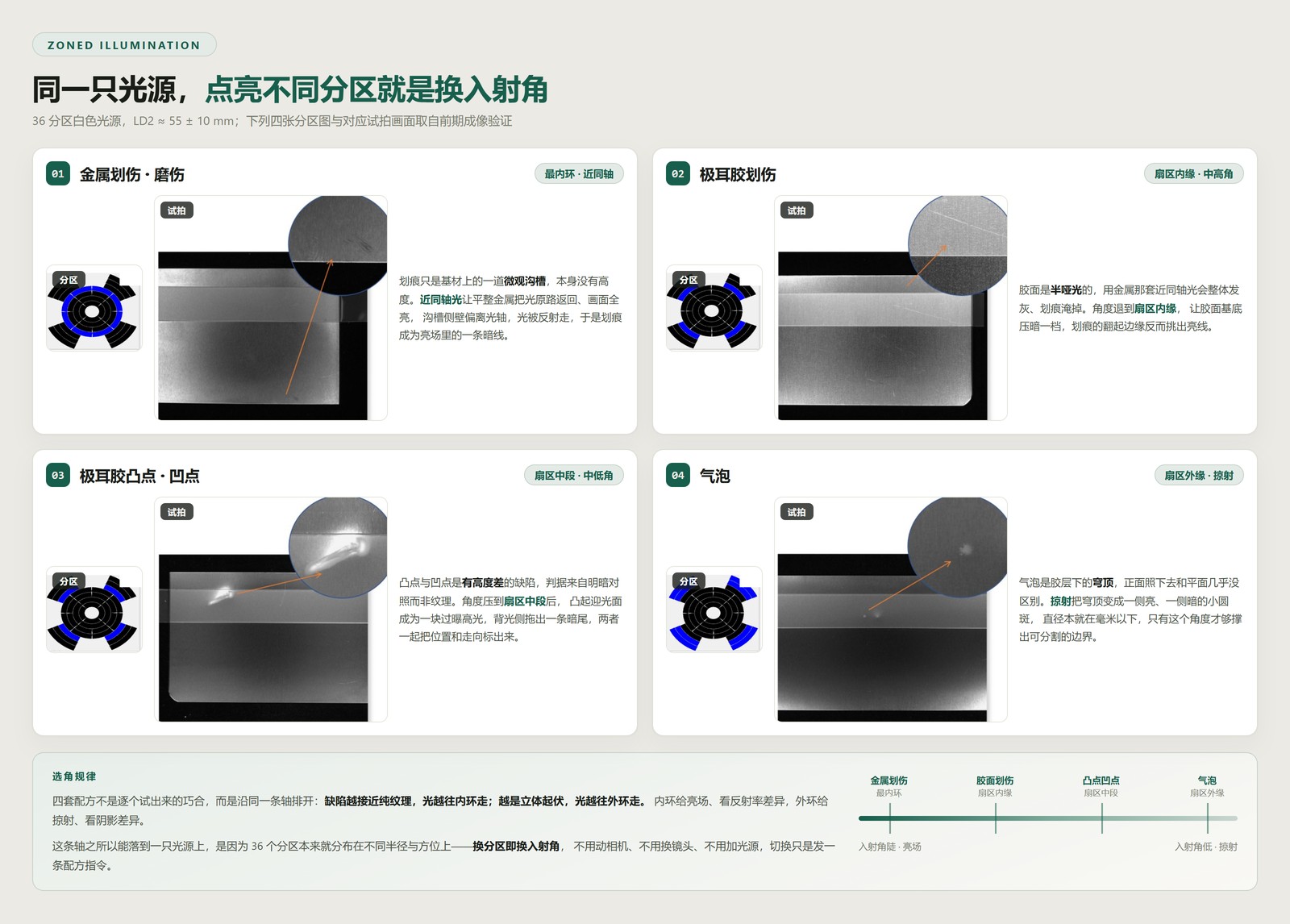
A lighting recipe is a reusable asset: a new product changes zone combinations and brightness, not the opto-mechanical design.
05/10Segmented Capture
A 68 mm field has to cover a 1410 mm edge
One frame covers about a twentieth of the long edge. 1410 ÷ 68 ≈ 20.7, so 21 segments without overlap and about 23 with a 10 % stitch margin. Each segment still needs one exposure per lighting recipe to cover all seven families, which puts a part at 84–92 exposures. That is where cycle time is decided—not in inference latency.
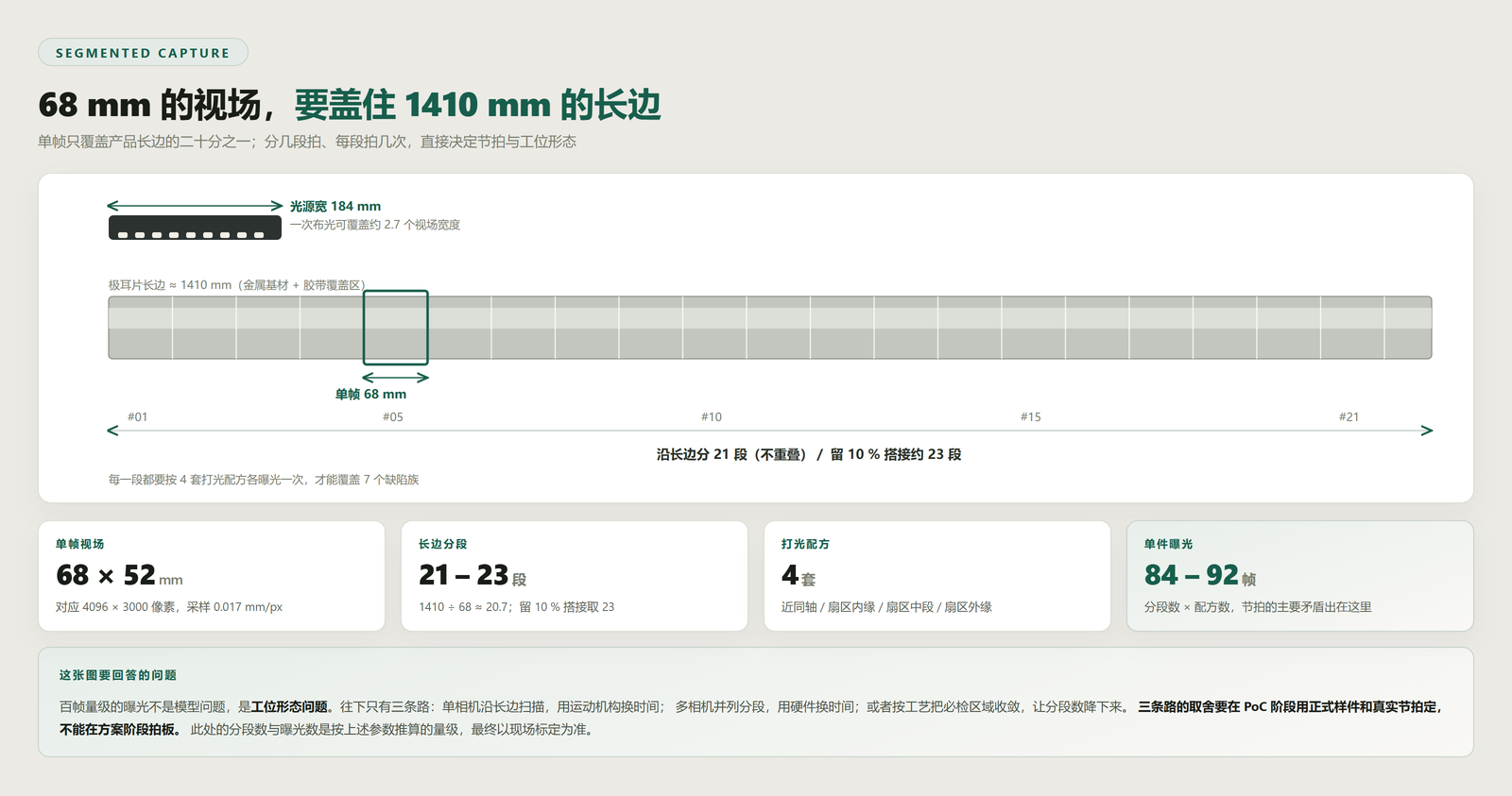
Exposures in the hundreds leave three routes: one camera scanning the edge, trading motion for time; several cameras in a row splitting the segments, trading hardware for time; or narrowing the mandatory inspection area by process agreement so the segment count drops. Each route has its own cost, and the choice has to be settled during PoC with official samples and real takt—not on paper. The segment and exposure figures here are magnitudes derived from the parameters above; the field calibration is what counts.
06/10Tensor Flow
Four recipes, four branches, one workflow
The vision agent runs on the edge: configuration, inference, HMI and outputs share one software stack, wired zero-code on a canvas—drag operators from the library, connect them by data flow. This project is not a single serial chain but four branches split by lighting recipe: each lights its zones, captures, segments and detects events; all four merge into one state machine, then save images and talk to the PLC over serial.
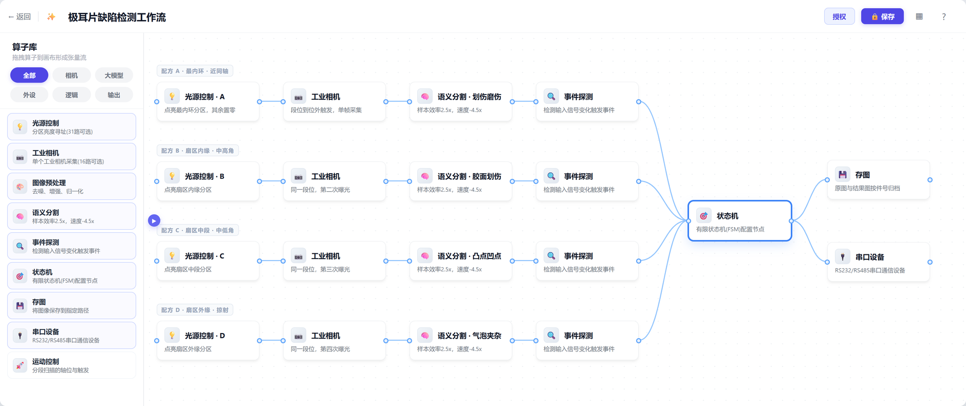
Double-click a node for its sub-editor: segmentation → annotate tool, event detection → GPU event composer, state machine → state-graph editor. A product change is mostly recipes and samples; moving the same flow to another size or station means editing zone combinations and thresholds, not rewriting line software.
07/10Segmentation
Pixel masks: lock a new defect with 1–10 samples
Tab defects rarely have regular boundaries: a scratch is a fine broken line, an inclusion is an arbitrary blob, an adhesive bump is a gradient bright patch. Boxes fit these poorly, and the grade decision downstream depends on contour size. The plan therefore uses pixel-level semantic segmentation: each class is defined in the annotate tool from a small set of line images—product guidance is 1–10 sample images and minutes of setup—and the resulting mask drives area, length or max bounding size.
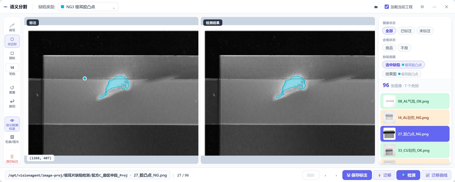
This is what makes “30 defect classes” affordable. A few-shot base means adding a class does not restart a collection-and-long-training cycle: between aluminium and copper, or between batches, similar morphologies often transfer with a handful of extra labels. Training and inference both run locally on the edge GPU, so station frames never leave the plant—good for latency and for data exposure alike.
08/10Events
Turning a mask into “inclusion over 0.5 mm”
Segmentation only sees pixels; the line needs decidable events. Events are composed in the GPU event composer: primitives such as object presence, width measurement and count are given a target class and a region, then combined with AND / OR / NOT. The inclusion grade lands here—object presence confirms the mask belongs to the inclusion family, and width measurement takes the mask's max bounding size against a millimetre threshold.
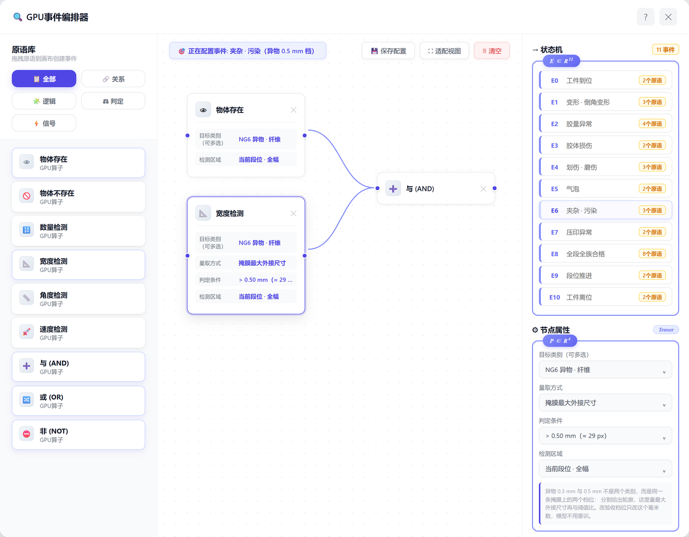
Keeping thresholds in the event layer rather than inside the model is the structural point. The 0.3 mm and 0.5 mm grades share one mask and one model, so changing the acceptance grade is a single millimetre edit. The same holds for adhesive-overrun tolerance and scratch-length limits: they live in the recipe, and perception stays untouched.
09/10State Machine
Scan segment by segment; release only when every segment and family is clear
Segmented capture creates a problem manual inspection never had: one part yields twenty-odd segments and a hundred-odd frames, and something has to fold them into a single verdict. The state machine encodes the floor process: once the part is in place it enters segmented scanning, self-loops after each segment finishes its four recipes and advances to the next. Only when every segment and every family is clear does it release and count; a hit in any family at any segment turns it NG, and the saved image carries the segment index and the class. An NG part leaves for review and, after re-judgement, re-enters the cycle.
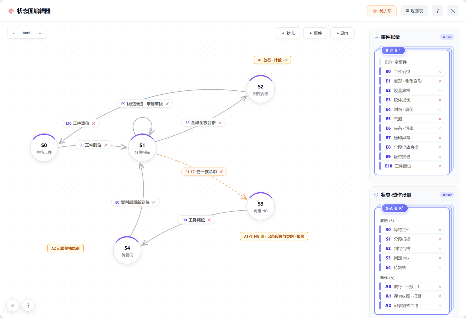
E9 (segment advance) self-loops S1 until the full length is scanned; E8 (all segments and families clear) takes the upper branch to release, while any of E1–E7 routes to NG with the evidence retained and the review verdict archived.The machine does not answer “does this frame look like a defect” but “may this part pass under the current recipe”—with the segment, the class and a reviewable record attached.
10Deployment
Edge-local inference, with samples and verdicts accumulating together
The system sits on five layers. Cameras and the zoned light capture; a gigabit industrial network keeps traffic inside the plant, so images never leave the site; the edge GPU runs segmentation, event decisions and the state machine; the front end provides live view, NG alarms, human review and retrieval by time, part ID or defect; recipes centrally manage camera parameters, zone combinations, model versions and thresholds. Raw frames, masks, result images and verdicts are archived per part—material for traceability, and the sample source for the next round of model tuning. The longer the line runs, the more usable samples exist, which is exactly the input continuous iteration needs.
Equipment list
The table fixes categories and configuration direction only; specific models freeze after official samples, mechanical space and cycle time are checked.
| # | Item | Configuration direction | Purpose |
|---|---|---|---|
| 1 | Industrial camera | 4096 × 3000, external trigger | Capture surface, edge and adhesive zones at 0.017 mm/pixel |
| 2 | Fixed-focus lens | 25 mm, WD ≈ 120 ± 10 mm | Match the 68 × 52 mm single-frame field |
| 3 | Zoned light | 36-zone white light, programmable per-zone brightness | Switch incidence angle by recipe across four morphologies |
| 4 | Motion or multi-camera segmentation | Sized to the 21–23 segment plan | Cover the 1410 mm long edge |
| 5 | Locating fixture | Repeatable positioning, quick clamping | Hold tab pose for imaging consistency |
| 6 | Presence sensor / PLC interface | Industrial DIO or fieldbus | Trigger capture, return results, gate the station |
| 7 | Edge computing unit | Sized for parallel multi-recipe inference and storage | Inference, metrology, HMI and archiving |
| 8 | HMI and alarm | Industrial monitor, tower light, buzzer | Display, alarm, review and operation |
Rollout
Staged delivery, each stage with an acceptable output:
| Stage | Duration | Main work | Output |
|---|---|---|---|
| Survey | 1 week | Site walk-through, sample confirmation, family cross-check, cycle-time and imaging assessment | Survey report · family confirmation sheet |
| Design | 1 week | Zone recipes, segmentation plan, inspection regions, model and rule design | Detailed design · deployment plan |
| Pilot | 2 weeks | Installation, camera calibration, sample labelling, recipe and event configuration, commissioning | Live system · configuration record · training material |
| Tuning | 2 weeks | Adjust thresholds and model against false-call and escape samples; stabilise takt and reporting | Tuning report · acceptance material · O&M manual |
| Replication | As needed | Extend to further sizes and stations; extend families and reports | Multi-size deployment · platform upgrade |
The boundary is explicit: this plan targets metal–adhesive composite surfaces with many similar-looking defect types and frequently moving tolerance grades. The cycle-time ceiling of segmented scanning is set by the mechanical design; where takt is tighter, it has to be balanced with parallel cameras or a narrower mandatory area. Defects inside the adhesive layer, and curled or badly warped parts that fall outside depth of field, need process support or an added orthogonal view. All parameters and segment magnitudes above come from the imaging validation and derivation; recognition rates and decision thresholds are confirmed on official samples in a fixed fixture.
blue
PhD in computer vision · VisionAgent solutions and delivery
Works on few-shot segmentation and industrial scene understanding; argues for moving appearance QC from “one long training run per defect” to “few-shot segmentation + event composition + state-machine aggregation”, so thresholds decouple from perception and a grade change needs no retraining.
Currently focused on edge GPU inference, cross-domain generalisation and closing the data loop on site. This piece records the family grouping, sampling derivation and platform configuration path behind a battery tab inspection plan.